Fourier-Mellin transform
The Fourier-Mellin transform of a function \(f(r, \theta)\) is given by: \[ M_f(\boldsymbol{u}, v) = \frac{1}{2\pi}\int_{0}^{\infty} \int_{0}^{2\pi} f(r, \theta)\boldsymbol{r^{-ju}}e^{-jv\theta}d\theta \boldsymbol{\frac{dr}{r}} \qquad [3] \]
where the elements in bold are the Mellin transform parameters and the remaining are the Fourier transform parameters. If two functions have a rotation and scale difference such that \(f_1(r, \theta) = f_2(\alpha r, \theta + \beta)\), then their Fourier-Mellin transforms are related as follows:
\[ M_{f_1}(u, v) = \alpha^{-ju}e^{jv\beta}M_{f_2}(u, v) \qquad [3] \]
where the magnitudes of \(M_{f_1}(u,v)\) and \(M_{f_2}(u,v)\) have a translation in the \(r\) and \(θ\) axes. By substituting \(r = e^{\rho}\), the FMT can be expressed as just a Fourier transformation:
\[ M_f(u, v) = \frac{1}{2\pi}\int_{-\infty}^{\infty} \int_{0}^{2\pi} f(e^\rho, \theta)e^{-ju\rho}e^{-jv\theta}d\theta d\rho \qquad [3] \]
Hence, by taking the Fourier transform of the input images and remapping to log-polar coordinates, rotation and scaling is expressed as translations in the resulting image (regardless of translations that might be present in the original image).
This can also be explained using the Fourier rotation and similarity theorems. Suppose two images are related by a translation and rotation: \[ f_2(x,y) = f_1(x\cos\theta + y\sin\theta - t_x, -x\sin\theta + y\cos\theta - t_y) \qquad [4] \]
In addition to the Fourier shift theorem, the Fourier rotation theorem is applied to get the following relationship between the Fourier transforms of the images: \[ F_2(\xi, \eta) = e^{-j2\pi(\xi t_x + \eta t_y)}F_1(\xi\cos\theta + \eta\sin\theta, -\xi\sin\theta + \eta\cos\theta) \]
As in the case with translated images, there is a phase difference of \(e^{-j2\pi(\xi t_x + \eta t_y)}\).
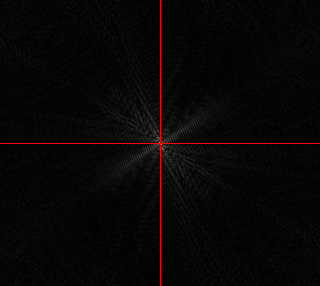
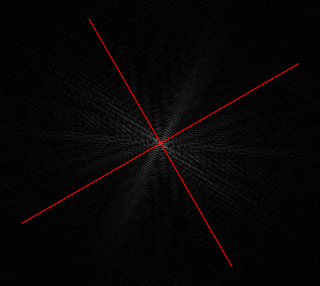
In addition, the magnitude of \(F_2\) is rotated by \(\theta\) with respect to the magnitude of \(F_1\). If the magnitude plots are converted to polar coordinates, the plots will be related by a translation.
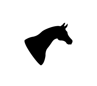
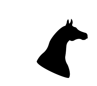
Using the same horse outline from earlier, we see that the magnitude plots of the second image are rotated by the same amount as the image itself (30 degrees in this case)
Similarly, if two images are related by a scaling factor:
\[ f_2(x,y) = f_1(\alpha x, \beta y) \]
then their Fourier transforms are related as:
\[ F_2(\xi, \eta) = \frac{1}{|\alpha\beta|}F_1(\frac{\xi}{\alpha}, \frac{\eta}{\beta}) \quad [5] \]
Also, if we assume there’s no skew between the images, we can set \(\alpha = \beta \). By converting the axes into the logarithmic scale, the scaling is represented as a translation:
\[ F_2(\log\xi, \log\eta) = F_1(\log\xi - \log\alpha, \log\eta - \log\alpha) \]
Since the scaling can also be represented by a translation, the phase correlation method can now be used to find the scale difference between the two images.
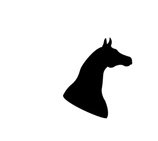
The horse outline below is scaled by 1.2 and rotated by 30 degrees relative to the reference image,
and the following images are the log-polar transformed magnitude plots of the two images:
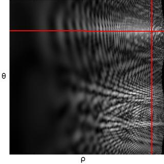
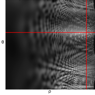
By performing phase correlation on the above two images, we get the following, with a peak at (11, -53):
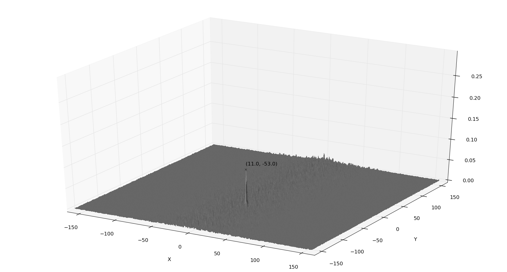
The log-polar images are translated by 11 and -53 pixels in x and y respectively. In order to calculate the rotation and scaling we use the following formulae:
\[ size = max(rows, cols) = max(286, 320) \] \[ \log_{base} \frac{rows}{2} = size \] \[ base = \exp^{\frac{\log \frac{rows}{2}}{size}} = \exp^{\frac{\log \frac{286}{2}}{320}} = 1.015 \] \[ \theta = \frac{-180 * row}{size} = \frac{-180 * -53}{320} = 29.81 \] \[ s = base^{col} = 1.015^{11} = 1.18 \]
We choose the log-polar image to be square with the size equal to the maximum dimension of the input images.
Once the second image has been derotated and scaled, any remaining translation between the two images can be estimated using the phase correlation method again.
[3] T. Kazik and A. H. Göktoğan, “Visual Odometry Based on the Fourier-Mellin Transform for a Rover Using a Monocular Ground-Facing Camera,” in Mechatronics (ICM), 2011 IEEE International Conference on, pp. 469–474, IEEE, 2011
[4] H. T. Ho and R. Goecke, “Optical Flow Estimation using Fourier Mellin Transform,” in Computer Vision and Pattern Recognition, 2008. CVPR 2008. IEEE Conference on, pp. 1–8, IEEE, 2008
[5] J. W. Goodman and S. C. Gustafson, Reviewer, “Introduction to Fourier Optics, Second Edition,” Optical Engineering, vol. 35, no. 5, pp. 1513–1513, 1996.